Capítol 6 Teoria Setmana 6

6.1 Packages

install.packages("VIM")

6.2 Barómetre (2021-01-29)

Anàlisis de la enquesta preelectoral. Perfil de votant al PSC segons la variable de intenció de vot.

library(foreign)
suppressPackageStartupMessages(library(tidyverse))
library(cowplot)
library(visreg)
library(scales)

data <- read.spss("http://upceo.ceo.gencat.cat/wsceop/7908/Microdades%20anonimitzades%20-992.sav", to.data.frame = TRUE, use.value.labels = TRUE)

data <- data %>% 
  select(P15R,PROVINCIA,HABITAT,SEXE,EDAT,P38)

dim(data)

## [1] 1100    6

Les variables seleccionades:

• P15R: En les eleccions al Parlament de Catalunya, convocades pel proper 14 de febrer - a quin partit o coalició votarà? (Agrupació partits)
• PROVINCIA
• HABITAT
• SEXE
• EDAT
• P38: Sumant els ingressos nets mensuals de totes les persones de la seva llar, - aproximadament, quins són els ingressos familiars que entren cada mes a casa seva

Veiem les freqüències de intenció de vot a cada partit.

table(data$P15R)

## 
##                     PPC                     ERC                     PSC                     C's                     CUP 
##                      14                     165                     116                      18                      42 
##                  PDeCAT     Junts per Catalunya Catalunya en Comú Podem                     Vox           Altres, blanc 
##                      11                      93                      49                      10                      28 
##                     Nul              No votaria                   NS/NC 
##                       4                      71                     479

data$Vot <- as.numeric(data$P15R == "PSC")
summary(data$Vot)

##    Min. 1st Qu.  Median    Mean 3rd Qu.    Max. 
##  0.0000  0.0000  0.0000  0.1055  0.0000  1.0000

S’observa un 10,6% en la intenció del vot del PSC.

6.2.1 Anàlisis univariant y bivariant

Carreguem funcions per establir els intervals de confiança basats en l’error estàndard.

errStd_bin <- function(x) { sqrt(mean(x)*(1-mean(x)) / length(x))}
minInt_bin <- function(x) { mean(x) - 1.96 *errStd_bin(x) }
maxInt_bin <- function(x) { mean(x) + 1.96 *errStd_bin(x) }

6.2.1.1 PROVINCIA

RESUM <- data %>% 
  group_by(PROVINCIA ) %>% 
  summarise(freq_absolutes = n()
         ,I_minim = minInt_bin(Vot )
         ,propensio = mean(Vot )
         ,I_maxim = maxInt_bin(Vot )) %>% 
  mutate(freq_relatives = freq_absolutes / sum(freq_absolutes))


p1 <- RESUM %>% 
  ggplot(aes(PROVINCIA , freq_relatives)) +
  geom_bar(stat="identity")+
  geom_text(aes(label = freq_absolutes), vjust=1.6, color="white")+
  scale_y_continuous(labels = percent)+
  theme_minimal()+
  theme(axis.text.x = element_text(angle = 90, vjust = 0.5, hjust=1))+
  labs(title="Freqüencies")

p2 <- RESUM %>% 
  ggplot(aes(PROVINCIA , propensio)) +
  geom_point(size = 1.5) +
  geom_errorbar(aes(ymin =I_minim, ymax = I_maxim, width = .2))+
  scale_y_continuous(labels = percent)+
  theme_minimal()+
  theme(axis.text.x = element_text(angle = 90, vjust = 0.5, hjust=1))+
  labs(title="Intervals confiança Indecisió")

plot_grid(p1, p2, ncol=2)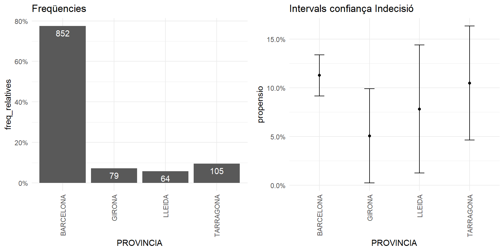

6.2.1.2 HABITAT

RESUM <- data %>% 
  group_by(HABITAT ) %>% 
  summarise(freq_absolutes = n()
         ,I_minim = minInt_bin(Vot )
         ,propensio = mean(Vot )
         ,I_maxim = maxInt_bin(Vot )) %>% 
  mutate(freq_relatives = freq_absolutes / sum(freq_absolutes))


p1 <- RESUM %>% 
  ggplot(aes(HABITAT , freq_relatives)) +
  geom_bar(stat="identity")+
  geom_text(aes(label = freq_absolutes), vjust=1.6, color="white")+
  scale_y_continuous(labels = percent)+
  theme_minimal()+
  theme(axis.text.x = element_text(angle = 90, vjust = 0.5, hjust=1))+
  labs(title="Freqüencies")

p2 <- RESUM %>% 
  ggplot(aes(HABITAT , propensio)) +
  geom_point(size = 1.5) +
  geom_errorbar(aes(ymin =I_minim, ymax = I_maxim, width = .2))+
  scale_y_continuous(labels = percent)+
  theme_minimal()+
  theme(axis.text.x = element_text(angle = 90, vjust = 0.5, hjust=1))+
  labs(title="Intervals confiança Indecisió")

plot_grid(p1, p2, ncol=2)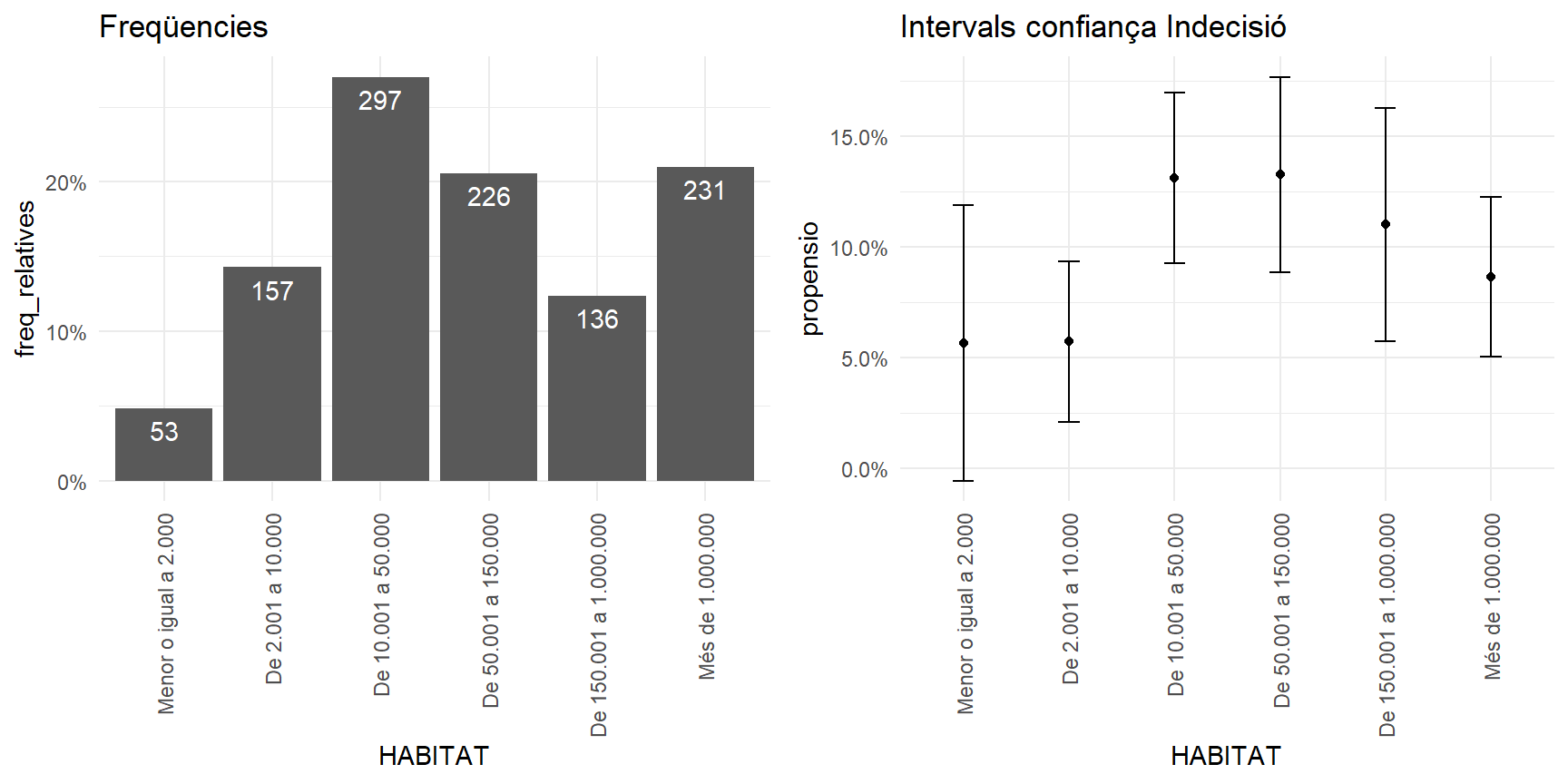

data <- data %>% 
  mutate(HABITAT_R = as.factor(ifelse(as.numeric(HABITAT)<=2,"3-Petita",
    ifelse(as.numeric(HABITAT)<=4,"2-Mitjana", "1-Gran"))))

RESUM <- data %>% 
  group_by(HABITAT_R ) %>% 
  summarise(freq_absolutes = n()
         ,I_minim = minInt_bin(Vot )
         ,propensio = mean(Vot )
         ,I_maxim = maxInt_bin(Vot )) %>% 
  mutate(freq_relatives = freq_absolutes / sum(freq_absolutes))


p1 <- RESUM %>% 
  ggplot(aes(HABITAT_R , freq_relatives)) +
  geom_bar(stat="identity")+
  geom_text(aes(label = freq_absolutes), vjust=1.6, color="white")+
  scale_y_continuous(labels = percent)+
  theme_minimal()+
  theme(axis.text.x = element_text(angle = 90, vjust = 0.5, hjust=1))+
  labs(title="Freqüencies")

p2 <- RESUM %>% 
  ggplot(aes(HABITAT_R , propensio)) +
  geom_point(size = 1.5) +
  geom_errorbar(aes(ymin =I_minim, ymax = I_maxim, width = .2))+
  scale_y_continuous(labels = percent)+
  theme_minimal()+
  theme(axis.text.x = element_text(angle = 90, vjust = 0.5, hjust=1))+
  labs(title="Intervals confiança Indecisió")

plot_grid(p1, p2, ncol=2)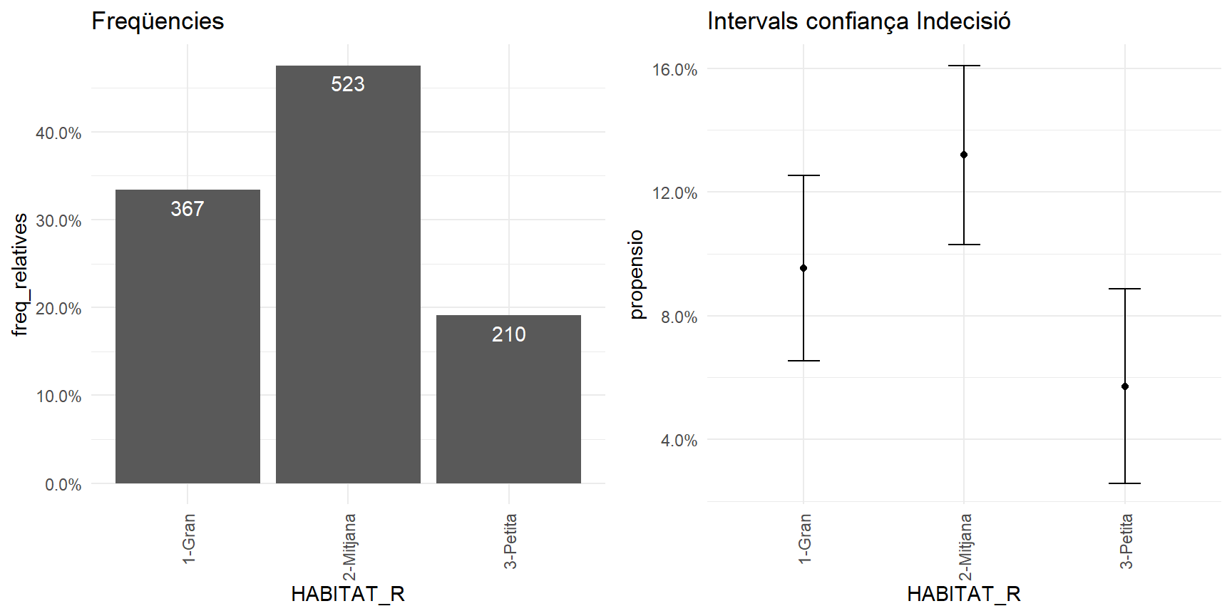

6.2.1.3 SEXE

RESUM <- data %>% 
  group_by(SEXE ) %>% 
  summarise(freq_absolutes = n()
         ,I_minim = minInt_bin(Vot )
         ,propensio = mean(Vot )
         ,I_maxim = maxInt_bin(Vot )) %>% 
  mutate(freq_relatives = freq_absolutes / sum(freq_absolutes))


p1 <- RESUM %>% 
  ggplot(aes(SEXE , freq_relatives)) +
  geom_bar(stat="identity")+
  geom_text(aes(label = freq_absolutes), vjust=1.6, color="white")+
  scale_y_continuous(labels = percent)+
  theme_minimal()+
  theme(axis.text.x = element_text(angle = 90, vjust = 0.5, hjust=1))+
  labs(title="Freqüencies")

p2 <- RESUM %>% 
  ggplot(aes(SEXE , propensio)) +
  geom_point(size = 1.5) +
  geom_errorbar(aes(ymin =I_minim, ymax = I_maxim, width = .2))+
  scale_y_continuous(labels = percent)+
  theme_minimal()+
  theme(axis.text.x = element_text(angle = 90, vjust = 0.5, hjust=1))+
  labs(title="Intervals confiança Indecisió")

plot_grid(p1, p2, ncol=2)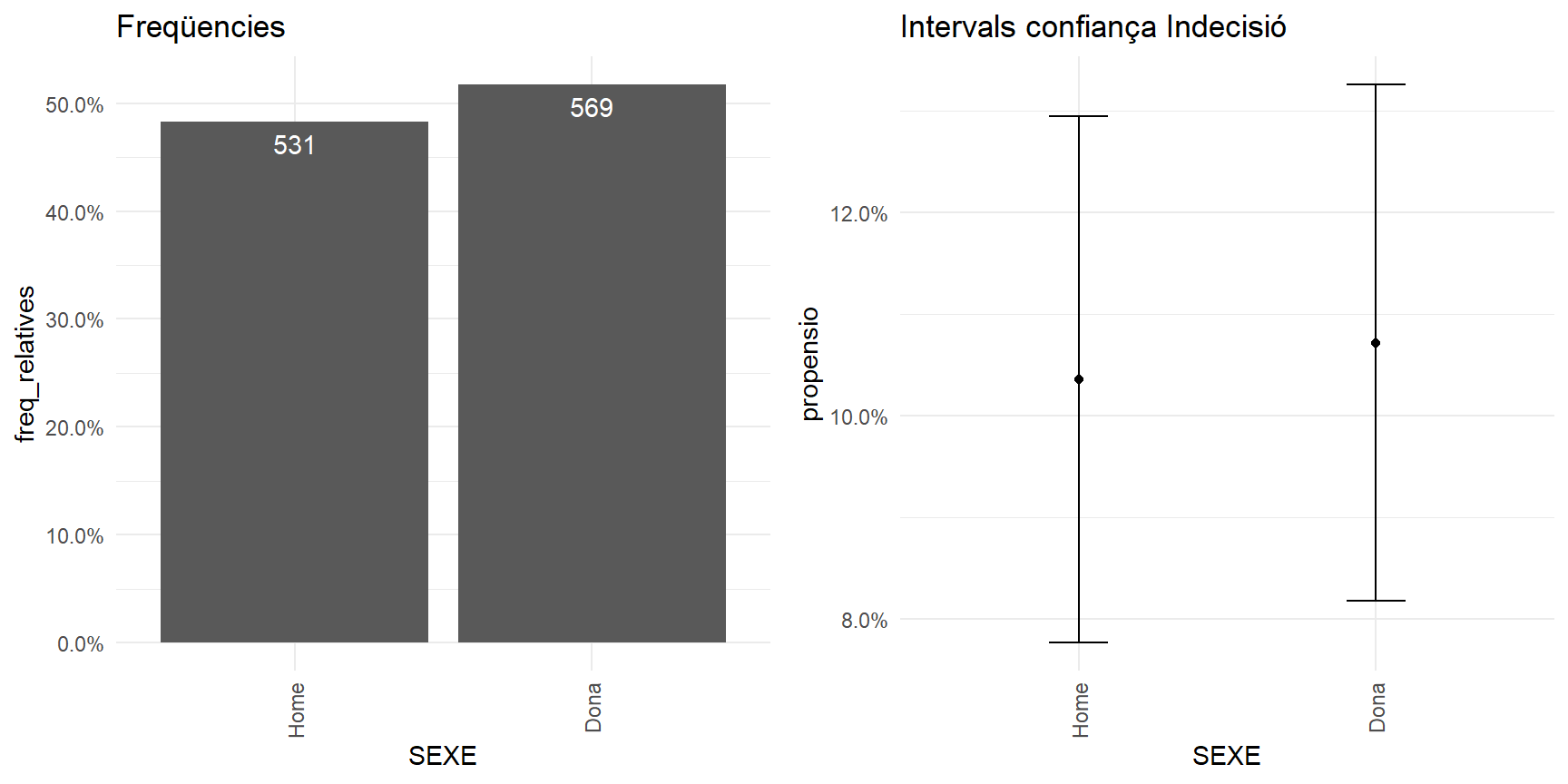

6.2.1.4 EDAT

summary(data$EDAT)

##    Min. 1st Qu.  Median    Mean 3rd Qu.    Max. 
##   18.00   38.00   51.00   51.08   65.00   98.00

data <- data %>% 
  mutate(EDAT_R = cut(EDAT,c(18,seq(25,85,10),100),include.lowest=TRUE))

RESUM <- data %>% 
  group_by(EDAT_R ) %>% 
  summarise(freq_absolutes = n()
         ,I_minim = minInt_bin(Vot )
         ,propensio = mean(Vot )
         ,I_maxim = maxInt_bin(Vot )) %>% 
  mutate(freq_relatives = freq_absolutes / sum(freq_absolutes))


p1 <- RESUM %>% 
  ggplot(aes(EDAT_R , freq_relatives)) +
  geom_bar(stat="identity")+
  geom_text(aes(label = freq_absolutes), vjust=1.6, color="white")+
  scale_y_continuous(labels = percent)+
  theme_minimal()+
  theme(axis.text.x = element_text(angle = 90, vjust = 0.5, hjust=1))+
  labs(title="Freqüencies")

p2 <- RESUM %>% 
  ggplot(aes(EDAT_R , propensio)) +
  geom_point(size = 1.5) +
  geom_errorbar(aes(ymin =I_minim, ymax = I_maxim, width = .2))+
  scale_y_continuous(labels = percent)+
  theme_minimal()+
  theme(axis.text.x = element_text(angle = 90, vjust = 0.5, hjust=1))+
  labs(title="Intervals confiança Indecisió")

plot_grid(p1, p2, ncol=2)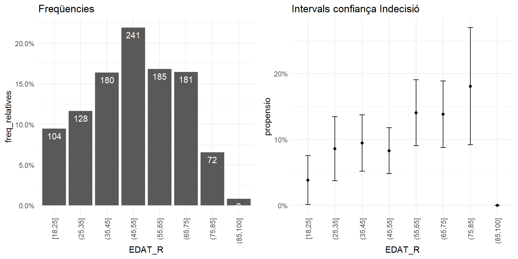

6.2.1.5 P38

RESUM <- data %>% 
  group_by(P38 ) %>% 
  summarise(freq_absolutes = n()
         ,I_minim = minInt_bin(Vot )
         ,propensio = mean(Vot )
         ,I_maxim = maxInt_bin(Vot )) %>% 
  mutate(freq_relatives = freq_absolutes / sum(freq_absolutes))

p1 <- RESUM %>% 
  ggplot(aes(P38 , freq_relatives)) +
  geom_bar(stat="identity")+
  geom_text(aes(label = freq_absolutes), vjust=1.6, color="white")+
  scale_y_continuous(labels = percent)+
  theme_minimal()+
  theme(axis.text.x = element_text(angle = 90, vjust = 0.5, hjust=1))+
  labs(title="Freqüencies")

p2 <- RESUM %>% 
  ggplot(aes(P38 , propensio)) +
  geom_point(size = 1.5) +
  geom_errorbar(aes(ymin =I_minim, ymax = I_maxim, width = .2))+
  scale_y_continuous(labels = percent)+
  theme_minimal()+
  theme(axis.text.x = element_text(angle = 90, vjust = 0.5, hjust=1))+
  labs(title="Intervals confiança Indecisió")

plot_grid(p1, p2, ncol=2)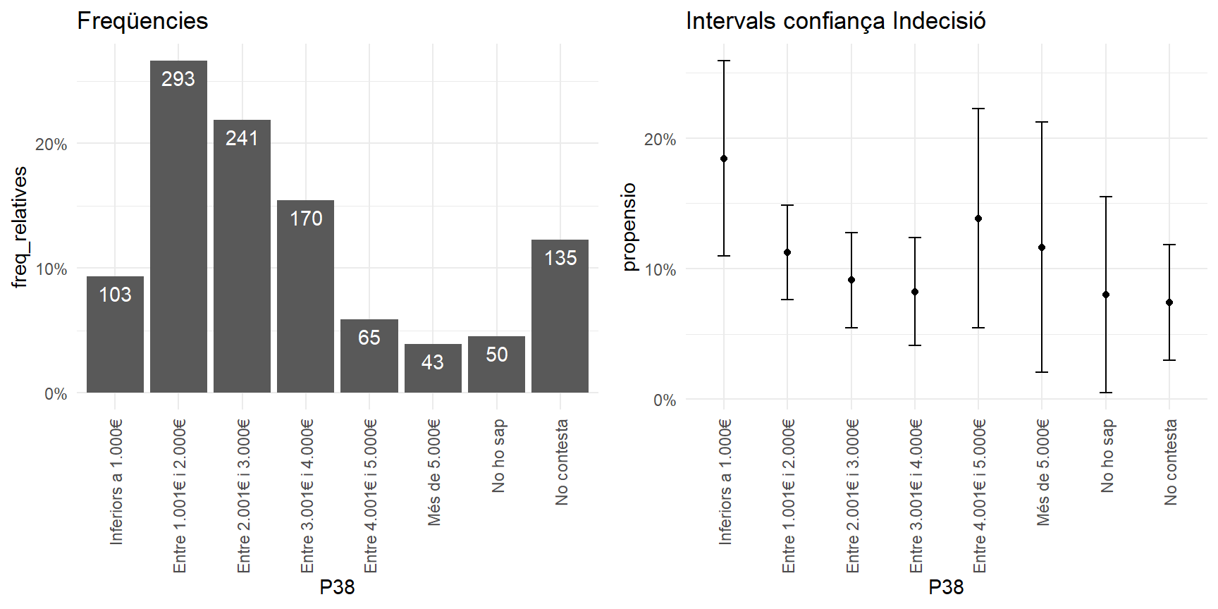

data$INGRES <- 500
data$INGRES[as.numeric(data$P38)==2] <- 1500
data$INGRES[as.numeric(data$P38)==3] <- 2500
data$INGRES[as.numeric(data$P38)==4] <- 3500
data$INGRES[as.numeric(data$P38)==5] <- 4500
data$INGRES[as.numeric(data$P38)==6] <- 5500

data$INGRES[data$P38=="No ho sap"]   <- 2500
data$INGRES[data$P38=="No contesta"] <- 2500

data$INGRES_NSNC <- "1-Contesta"
data$INGRES_NSNC[data$P38=="No ho sap"] <- "2-No ho sap"
data$INGRES_NSNC[data$P38=="No contesta"] <- "3-No contesta"

6.2.2

lreg1 <- glm(Vot ~ PROVINCIA + HABITAT_R + SEXE + EDAT + log(INGRES) + INGRES_NSNC, family=binomial, data= data) 

summary(lreg1)

## 
## Call:
## glm(formula = Vot ~ PROVINCIA + HABITAT_R + SEXE + EDAT + log(INGRES) + 
##     INGRES_NSNC, family = binomial, data = data)
## 
## Deviance Residuals: 
##     Min       1Q   Median       3Q      Max  
## -0.8683  -0.5224  -0.4229  -0.3362   2.5494  
## 
## Coefficients:
##                           Estimate Std. Error z value Pr(>|z|)   
## (Intercept)              -1.386826   1.376850  -1.007  0.31382   
## PROVINCIAGIRONA          -0.848774   0.539140  -1.574  0.11542   
## PROVINCIALLEIDA          -0.284928   0.506240  -0.563  0.57355   
## PROVINCIATARRAGONA       -0.048425   0.355967  -0.136  0.89179   
## HABITAT_R2-Mitjana        0.462629   0.230201   2.010  0.04447 * 
## HABITAT_R3-Petita        -0.402917   0.374768  -1.075  0.28233   
## SEXEDona                 -0.055966   0.203841  -0.275  0.78366   
## EDAT                      0.019331   0.006106   3.166  0.00155 **
## log(INGRES)              -0.238617   0.164638  -1.449  0.14724   
## INGRES_NSNC2-No ho sap   -0.160915   0.546105  -0.295  0.76825   
## INGRES_NSNC3-No contesta -0.515066   0.354438  -1.453  0.14617   
## ---
## Signif. codes:  0 '***' 0.001 '**' 0.01 '*' 0.05 '.' 0.1 ' ' 1
## 
## (Dispersion parameter for binomial family taken to be 1)
## 
##     Null deviance: 741.19  on 1099  degrees of freedom
## Residual deviance: 710.51  on 1089  degrees of freedom
## AIC: 732.51
## 
## Number of Fisher Scoring iterations: 5

100*(exp(coef(lreg1)) -1 )

##              (Intercept)          PROVINCIAGIRONA          PROVINCIALLEIDA       PROVINCIATARRAGONA       HABITAT_R2-Mitjana 
##               -75.013286               -57.206062               -24.793186                -4.727075                58.824328 
##        HABITAT_R3-Petita                 SEXEDona                     EDAT              log(INGRES)   INGRES_NSNC2-No ho sap 
##               -33.163210                -5.442899                 1.951906               -21.228365               -14.863541 
## INGRES_NSNC3-No contesta 
##               -40.253907

6.2.3 Regressió logística amb covariants: gràfic d’efectes condicionats

visreg(lreg1, "EDAT", 
       by = "HABITAT_R",
       cond=list(INGRES =500,SEXE="Home",PROVINCIA="BARCELONA"),  # condicionem a ser home
       band = TRUE,    # viualitzem bandes
       gg = TRUE,      # usem ggplot2
       overlay=TRUE,   # un mateix grafic
       scale="response") +
  labs(y = "Prob(Vot)", 
       x = "EDAT")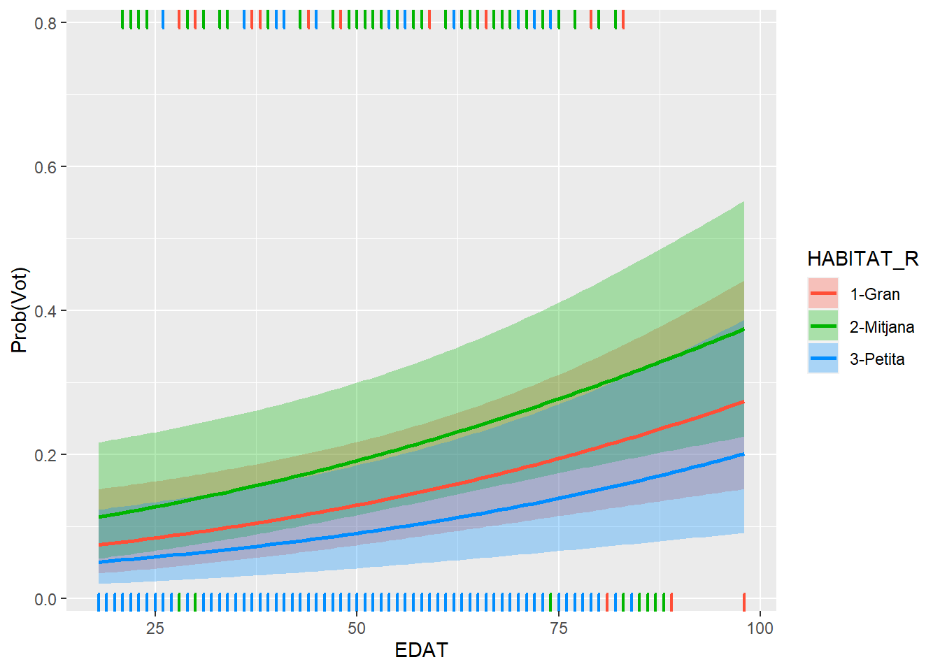

Observem com els homes, de Barcelona, amb ingressos nets mensuals de la llar igual a 500, en poblacions mitjanes, tenen una corba de probabilitat de Vots al PSC superior als altres mides d’hàbitat

6.3 PCA - Anàlisis de Components principals

d <- read.csv("www/data/mesa2021.csv", fileEncoding = "utf-8")

dim(d)

## [1] 9139   67

d<- d %>% 
  mutate(N_PSC=Vots.PARTIT.DELS.SOCIALISTES.DE.CATALUNYA..PSC.PSOE...PSC.
    ,N_ERC=Vots.ESQUERRA.REPUBLICANA.DE.CATALUNYA..ERC.
    ,N_JxCat=Vots.JUNTS.PER.CATALUNYA..JxCat.
    ,N_VOX=Vots.VOX..VOX.
    ,N_CUP=Vots.CANDIDATURA.D.UNITAT.POPULAR.UN.NOU.CICLE.PER.GUANYAR..CUP.G.
    ,N_COMUNS=Vots.EN.COMÚ.PODEM.PODEM.EN.COMÚ..ECP.PEC.
    ,N_Cs=Vots.CIUTADANS...PARTIDO.DE.LA.CIUDADANÍA..Cs.
    ,N_PP=Vots.PARTIT.POPULAR.PARTIDO.POPULAR..PP.
    ,N_TOT = N_PSC + N_ERC + N_JxCat + N_VOX + N_CUP + N_COMUNS + N_Cs + N_PP
    ,municipi=Nom.municipi,comarca=Nom.comarca)

dmesa<-d %>% 
  filter(N_TOT>0) %>% 
  mutate(PSC = N_PSC / N_TOT
         ,ERC = N_ERC  / N_TOT
         ,JxCat = N_JxCat  / N_TOT
         ,VOX = N_VOX  / N_TOT
         ,CUP = N_CUP  / N_TOT
         ,COMUNS = N_COMUNS  / N_TOT
         ,Cs = N_Cs  / N_TOT
         ,PP = N_PP  / N_TOT
         ) %>% 
  select(Districte,Secció,Mesa,municipi,comarca,PSC,ERC,JxCat,VOX,CUP,COMUNS,Cs,PP)

dmun <- d %>% 
  filter(N_TOT>0) %>% 
  group_by(municipi,comarca) %>% 
  summarise(PSC = sum(N_PSC) / sum(N_TOT)
         ,ERC = sum(N_ERC)  / sum(N_TOT)
         ,JxCat = sum(N_JxCat)  / sum(N_TOT)
         ,VOX = sum(N_VOX)  / sum(N_TOT)
         ,CUP = sum(N_CUP)  / sum(N_TOT)
         ,COMUNS = sum(N_COMUNS)  / sum(N_TOT)
         ,Cs = sum(N_Cs)  / sum(N_TOT)
         ,PP = sum(N_PP)  / sum(N_TOT)
         ) %>% 
  ungroup()

dcom <- d %>% 
  filter(N_TOT>0) %>% 
  group_by(comarca) %>% 
  summarise(PSC = sum(N_PSC) / sum(N_TOT)
         ,ERC = sum(N_ERC)  / sum(N_TOT)
         ,JxCat = sum(N_JxCat)  / sum(N_TOT)
         ,VOX = sum(N_VOX)  / sum(N_TOT)
         ,CUP = sum(N_CUP)  / sum(N_TOT)
         ,COMUNS = sum(N_COMUNS)  / sum(N_TOT)
         ,Cs = sum(N_Cs)  / sum(N_TOT)
         ,PP = sum(N_PP)  / sum(N_TOT)
         ) %>% 
  ungroup()

dim(dmesa)

## [1] 9139   13

head(dmesa)

##   Districte Secció Mesa municipi        comarca       PSC       ERC      JxCat        VOX        CUP     COMUNS         Cs
## 1         1      1    A   Abrera Baix Llobregat 0.3015075 0.2361809 0.10050251 0.07537688 0.06532663 0.10552764 0.07537688
## 2         1      1    B   Abrera Baix Llobregat 0.3898305 0.1807910 0.07344633 0.07344633 0.02259887 0.12994350 0.10734463
## 3         1      1    C   Abrera Baix Llobregat 0.2949309 0.2534562 0.07373272 0.11520737 0.05529954 0.07834101 0.08294931
## 4         1      2    A   Abrera Baix Llobregat 0.3594470 0.2119816 0.12903226 0.10138249 0.03225806 0.06451613 0.04608295
## 5         1      2    B   Abrera Baix Llobregat 0.4136364 0.1590909 0.05909091 0.09545455 0.03181818 0.10454545 0.07727273
## 6         1      2    C   Abrera Baix Llobregat 0.3756098 0.2097561 0.06341463 0.09756098 0.01951220 0.11219512 0.10243902
##           PP
## 1 0.04020101
## 2 0.02259887
## 3 0.04608295
## 4 0.05529954
## 5 0.05909091
## 6 0.01951220

X_mesa <- dmesa %>%
  select(PSC,ERC,JxCat,VOX,CUP,COMUNS,Cs,PP) %>% 
  scale()

head(X_mesa)

##            PSC        ERC      JxCat        VOX         CUP     COMUNS         Cs           PP
## [1,] 0.4798992  0.1872116 -0.8357312 -0.1714520 -0.09972564  0.9452201  0.5237459 -0.001549926
## [2,] 1.2818016 -0.6216485 -1.0546477 -0.2135402 -1.15370367  1.6421690  1.5415819 -0.626328468
## [3,] 0.4201883  0.4394833 -1.0523304  0.6968941 -0.34706685  0.1691800  0.7648478  0.207226599
## [4,] 1.0059435 -0.1661717 -0.6048918  0.3954972 -0.91543754 -0.2254502 -0.4089574  0.534364619
## [5,] 1.4979398 -0.9385347 -1.1708000  0.2662619 -0.92628825  0.9171837  0.5841085  0.668937304
## [6,] 1.1526885 -0.1986702 -1.1358159  0.3121843 -1.22984357  1.1355429  1.3853900 -0.735888375

round(cov(X_mesa),3)

##           PSC    ERC  JxCat    VOX    CUP COMUNS     Cs     PP
## PSC     1.000 -0.636 -0.880  0.560 -0.679  0.465  0.642  0.269
## ERC    -0.636  1.000  0.444 -0.562  0.418 -0.327 -0.607 -0.494
## JxCat  -0.880  0.444  1.000 -0.641  0.601 -0.577 -0.705 -0.343
## VOX     0.560 -0.562 -0.641  1.000 -0.636  0.120  0.623  0.431
## CUP    -0.679  0.418  0.601 -0.636  1.000 -0.217 -0.643 -0.414
## COMUNS  0.465 -0.327 -0.577  0.120 -0.217  1.000  0.315  0.027
## Cs      0.642 -0.607 -0.705  0.623 -0.643  0.315  1.000  0.461
## PP      0.269 -0.494 -0.343  0.431 -0.414  0.027  0.461  1.000

pca_mesa <- princomp(X_mesa)

summary(pca_mesa)

## Importance of components:
##                           Comp.1    Comp.2     Comp.3     Comp.4     Comp.5     Comp.6     Comp.7       Comp.8
## Standard deviation     2.1382945 1.0874848 0.84995171 0.71172482 0.60738263 0.57990364 0.55679971 1.703416e-08
## Proportion of Variance 0.5716005 0.1478441 0.09031212 0.06332596 0.04611925 0.04204063 0.03875748 3.627428e-17
## Cumulative Proportion  0.5716005 0.7194446 0.80975668 0.87308264 0.91920189 0.96124252 1.00000000 1.000000e+00

attributes(pca_mesa)

## $names
## [1] "sdev"     "loadings" "center"   "scale"    "n.obs"    "scores"   "call"    
## 
## $class
## [1] "princomp"

Z <- pca_mesa$scores

head(Z)

##         Comp.1     Comp.2      Comp.3      Comp.4     Comp.5     Comp.6     Comp.7        Comp.8
## [1,] 0.8665642  1.0070506 -0.06690843 -0.52329933 -0.1046999 -0.2737614  0.2039157 -3.053113e-16
## [2,] 2.3363692  1.7464017  0.15773682 -0.02917238  0.8176058 -0.8564416 -0.2182054  1.665335e-16
## [3,] 1.2282605  0.1575983  0.65913566 -0.50013781 -0.6020300 -0.2846055  0.2797815  3.330669e-16
## [4,] 1.1250577 -0.2502562  0.49254384 -0.21954622  0.3997918  1.0098184  0.3236403 -8.187895e-16
## [5,] 2.4677055  0.5828516 -0.28712250 -0.17836744  0.4988533  0.4020623  0.3165207 -9.020562e-16
## [6,] 2.1867538  1.3674877  0.81059413 -0.02288879  0.4167371 -0.6999940 -0.2129415  1.942890e-16

round(cov(Z),3)

##        Comp.1 Comp.2 Comp.3 Comp.4 Comp.5 Comp.6 Comp.7 Comp.8
## Comp.1  4.573  0.000  0.000  0.000  0.000  0.000   0.00      0
## Comp.2  0.000  1.183  0.000  0.000  0.000  0.000   0.00      0
## Comp.3  0.000  0.000  0.722  0.000  0.000  0.000   0.00      0
## Comp.4  0.000  0.000  0.000  0.507  0.000  0.000   0.00      0
## Comp.5  0.000  0.000  0.000  0.000  0.369  0.000   0.00      0
## Comp.6  0.000  0.000  0.000  0.000  0.000  0.336   0.00      0
## Comp.7  0.000  0.000  0.000  0.000  0.000  0.000   0.31      0
## Comp.8  0.000  0.000  0.000  0.000  0.000  0.000   0.00      0

6.3.1 Components Principals: gràfics d’individus, variables

plot(pca_mesa$scores[,1:2], pch =".", main ="Gràfic de meses")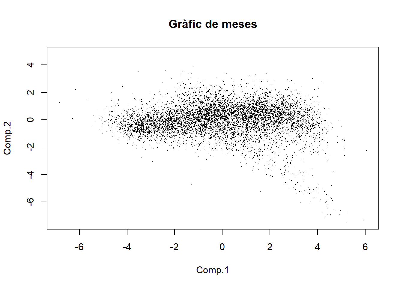

biplot(pca_mesa, cex=0.7, col=c("grey","red"))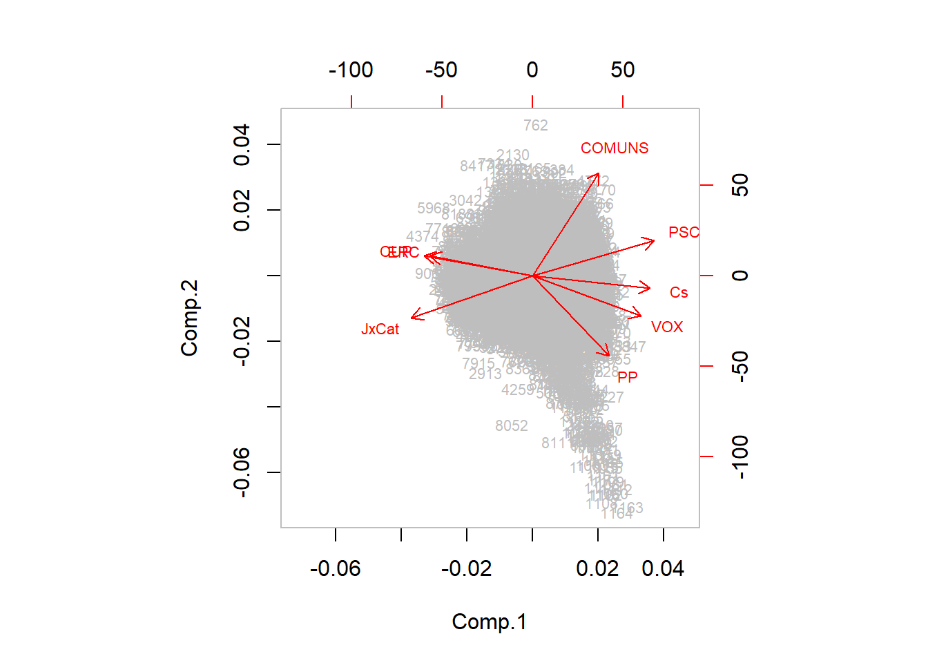

library(FactoMineR)

respca_mesa <- PCA(X_mesa, graph=FALSE)
summary(respca_mesa)

## 
## Call:
## PCA(X = X_mesa, graph = FALSE) 
## 
## 
## Eigenvalues
##                        Dim.1   Dim.2   Dim.3   Dim.4   Dim.5   Dim.6   Dim.7   Dim.8
## Variance               4.573   1.183   0.722   0.507   0.369   0.336   0.310   0.000
## % of var.             57.160  14.784   9.031   6.333   4.612   4.204   3.876   0.000
## Cumulative % of var.  57.160  71.944  80.976  87.308  91.920  96.124 100.000 100.000
## 
## Individuals (the 10 first)
##            Dist    Dim.1    ctr   cos2    Dim.2    ctr   cos2    Dim.3    ctr   cos2  
## 1      |  1.473 |  0.867  0.002  0.346 |  1.007  0.009  0.467 |  0.067  0.000  0.002 |
## 2      |  3.160 |  2.336  0.013  0.547 |  1.746  0.028  0.305 | -0.158  0.000  0.002 |
## 3      |  1.655 |  1.228  0.004  0.551 |  0.158  0.000  0.009 | -0.659  0.007  0.159 |
## 4      |  1.704 |  1.125  0.003  0.436 | -0.250  0.001  0.022 | -0.493  0.004  0.084 |
## 5      |  2.656 |  2.468  0.015  0.863 |  0.583  0.003  0.048 |  0.287  0.001  0.012 |
## 6      |  2.832 |  2.187  0.011  0.596 |  1.368  0.017  0.233 | -0.811  0.010  0.082 |
## 7      |  1.853 |  1.516  0.005  0.669 |  0.494  0.002  0.071 | -0.579  0.005  0.098 |
## 8      |  2.120 |  1.125  0.003  0.282 |  1.519  0.021  0.514 | -0.817  0.010  0.149 |
## 9      |  2.081 |  1.794  0.008  0.744 | -0.930  0.008  0.200 | -0.106  0.000  0.003 |
## 10     |  3.078 |  2.796  0.019  0.825 | -0.603  0.003  0.038 | -0.581  0.005  0.036 |
## 
## Variables
##           Dim.1    ctr   cos2    Dim.2    ctr   cos2    Dim.3    ctr   cos2  
## PSC    |  0.877 16.804  0.768 |  0.256  5.524  0.065 | -0.123  2.099  0.015 |
## ERC    | -0.744 12.107  0.554 |  0.143  1.718  0.020 | -0.449 27.900  0.202 |
## JxCat  | -0.878 16.851  0.771 | -0.302  7.730  0.091 |  0.138  2.627  0.019 |
## VOX    |  0.782 13.381  0.612 | -0.291  7.158  0.085 | -0.240  8.000  0.058 |
## CUP    | -0.786 13.509  0.618 |  0.145  1.781  0.021 |  0.375 19.478  0.141 |
## COMUNS |  0.477  4.969  0.227 |  0.745 46.976  0.556 |  0.339 15.888  0.115 |
## Cs     |  0.848 15.725  0.719 | -0.091  0.702  0.008 | -0.016  0.034  0.000 |
## PP     |  0.552  6.655  0.304 | -0.580 28.411  0.336 |  0.416 23.974  0.173 |

plot(respca_mesa,choix="ind", cex=.1)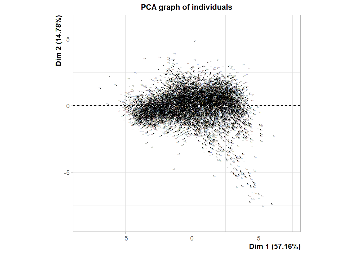

plot(respca_mesa,choix="var")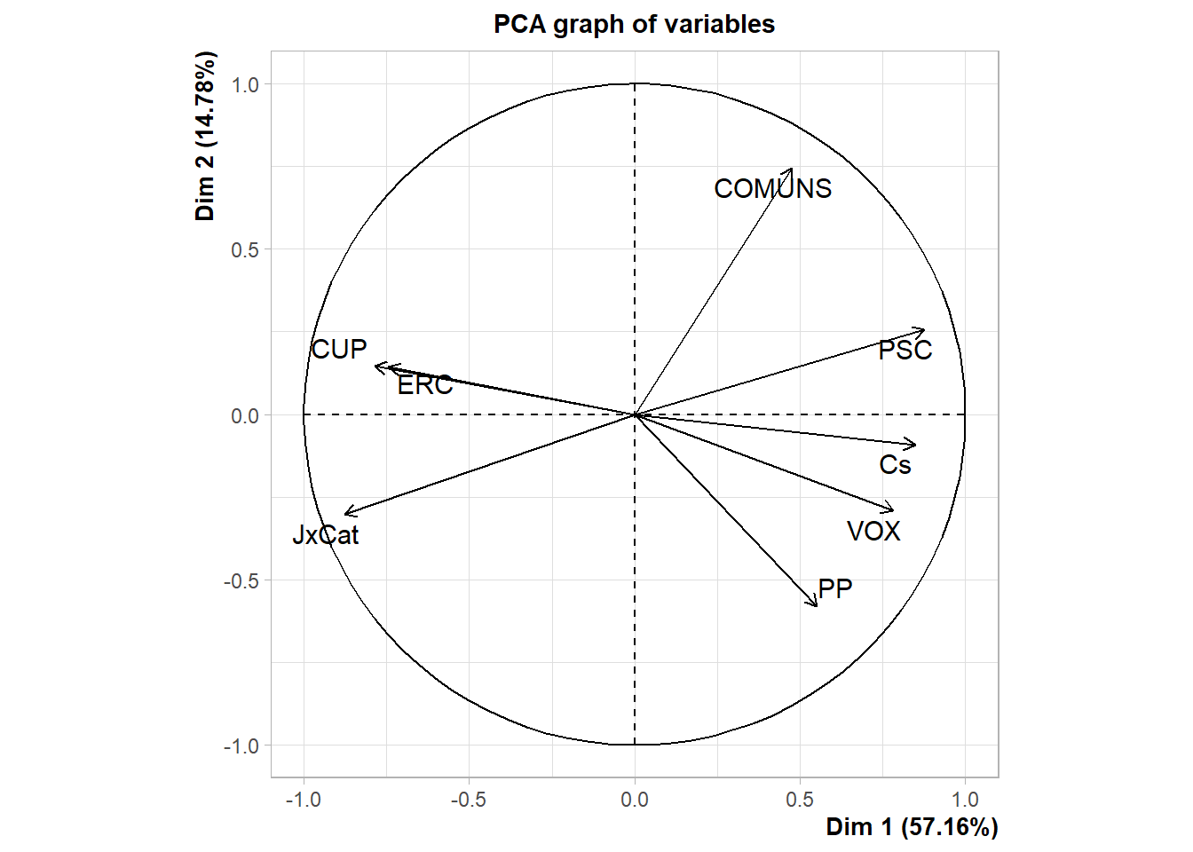

6.3.1.1 Muncipi

X_mun  <- dmun %>%
  select(PSC,ERC,JxCat,VOX,CUP,COMUNS,Cs,PP) %>% 
  scale()

head(X_mun)

##             PSC        ERC      JxCat         VOX        CUP     COMUNS         Cs          PP
## [1,] -1.0680025 -0.1951766  1.2652455 -1.26203775  0.8570902 -0.3219951 -0.5406946 -1.15890625
## [2,]  2.5592264 -1.0298304 -2.0999427  1.66838562 -1.2687628  1.7333943  2.4578172  0.65668030
## [3,] -0.3023732  0.2965304  0.3265143 -0.45103561  0.3688814 -0.9039498 -0.1663473 -0.46674009
## [4,] -0.3624323  0.5467015  0.5774023 -0.05130109 -0.9667080 -0.7251911 -0.2552742  0.02885896
## [5,] -1.1867827 -1.2967095  0.9280739 -0.43047329  2.8021293 -1.0867382 -0.6788765 -0.52016231
## [6,] -0.5559249  0.3756069 -0.2751672 -0.05149017  1.0593011  0.1636361  0.4630548 -0.88542106

respca_mun <- PCA(X_mun, graph=FALSE)

summary(respca_mun)

## 
## Call:
## PCA(X = X_mun, graph = FALSE) 
## 
## 
## Eigenvalues
##                        Dim.1   Dim.2   Dim.3   Dim.4   Dim.5   Dim.6   Dim.7   Dim.8
## Variance               4.073   1.110   1.022   0.738   0.498   0.296   0.261   0.000
## % of var.             50.914  13.880  12.775   9.231   6.231   3.706   3.262   0.000
## Cumulative % of var.  50.914  64.795  77.569  86.800  93.032  96.738 100.000 100.000
## 
## Individuals (the 10 first)
##            Dist    Dim.1    ctr   cos2    Dim.2    ctr   cos2    Dim.3    ctr   cos2  
## 1      |  2.618 | -2.365  0.145  0.816 |  0.864  0.071  0.109 |  0.295  0.009  0.013 |
## 2      |  5.091 |  4.994  0.647  0.962 |  0.234  0.005  0.002 |  0.676  0.047  0.018 |
## 3      |  1.300 | -1.078  0.030  0.688 | -0.185  0.003  0.020 | -0.189  0.004  0.021 |
## 4      |  1.515 | -0.554  0.008  0.134 | -0.808  0.062  0.285 | -0.966  0.096  0.407 |
## 5      |  3.730 | -2.397  0.149  0.413 |  2.182  0.453  0.342 |  0.044  0.000  0.000 |
## 6      |  1.637 | -0.525  0.007  0.103 |  0.160  0.002  0.010 |  1.079  0.120  0.435 |
## 7      |  0.563 | -0.391  0.004  0.483 | -0.236  0.005  0.176 |  0.208  0.004  0.136 |
## 8      |  1.429 |  0.326  0.003  0.052 |  0.278  0.007  0.038 |  1.351  0.189  0.894 |
## 9      |  1.803 | -0.956  0.024  0.282 |  1.130  0.121  0.393 | -0.715  0.053  0.157 |
## 10     |  5.334 |  1.634  0.069  0.094 | -1.846  0.324  0.120 | -2.541  0.667  0.227 |
## 
## Variables
##           Dim.1    ctr   cos2    Dim.2    ctr   cos2    Dim.3    ctr   cos2  
## PSC    |  0.899 19.850  0.809 | -0.040  0.143  0.002 |  0.096  0.899  0.009 |
## ERC    | -0.379  3.522  0.143 | -0.886 70.691  0.785 |  0.240  5.645  0.058 |
## JxCat  | -0.808 16.030  0.653 |  0.323  9.397  0.104 | -0.385 14.487  0.148 |
## VOX    |  0.843 17.452  0.711 |  0.021  0.040  0.000 | -0.179  3.148  0.032 |
## CUP    | -0.580  8.257  0.336 |  0.385 13.349  0.148 |  0.416 16.953  0.173 |
## COMUNS |  0.586  8.444  0.344 |  0.233  4.868  0.054 |  0.622 37.898  0.387 |
## Cs     |  0.881 19.074  0.777 |  0.092  0.754  0.008 | -0.029  0.081  0.001 |
## PP     |  0.548  7.370  0.300 | -0.092  0.757  0.008 | -0.462 20.890  0.213 |

plot(respca_mun,choix="ind", cex=.1)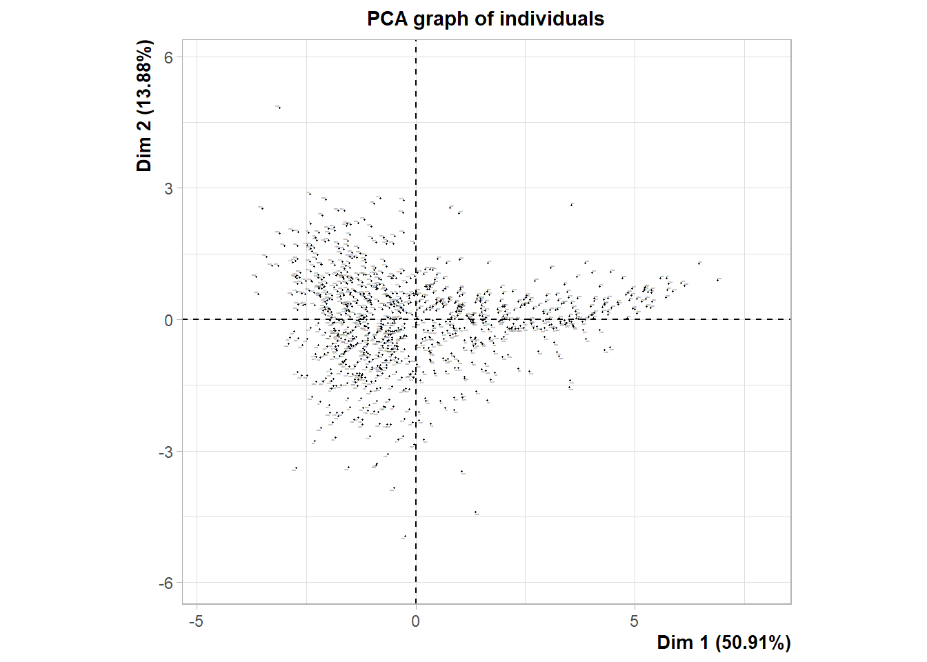

plot(respca_mun,choix="var")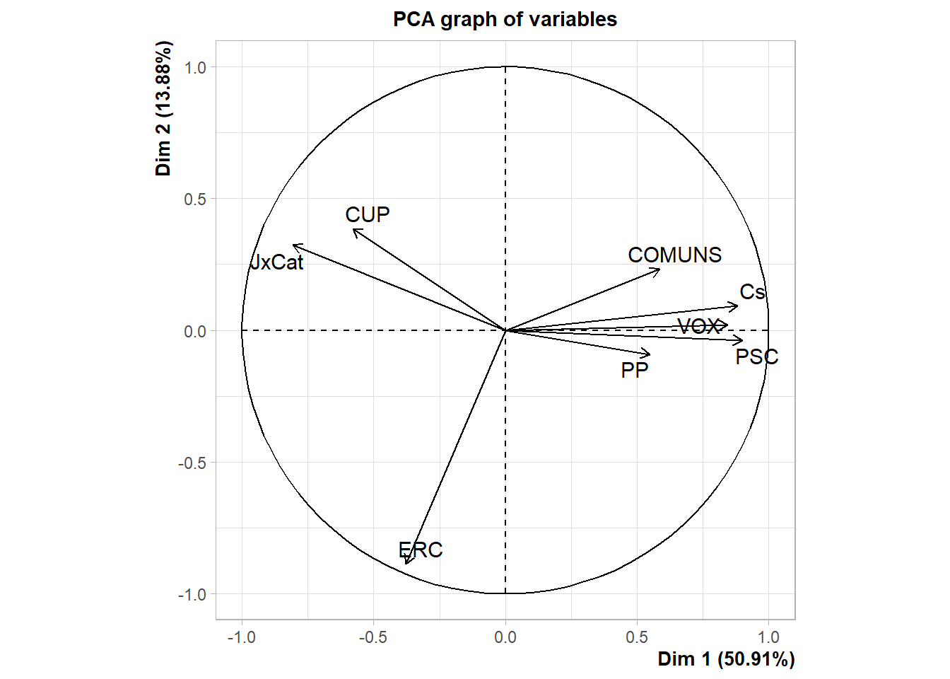

6.3.1.2 Comarca

X_com  <- dcom %>%
  select(PSC,ERC,JxCat,VOX,CUP,COMUNS,Cs,PP) %>% 
  scale()

rownames(X_com) <- dcom$comarca

head(X_com)

##                        PSC         ERC       JxCat          VOX         CUP     COMUNS         Cs           PP
## Alt Camp       -0.30529296  0.03487542  0.14640166  0.007228997  0.80049453 -0.5813202 -0.1443124 -0.250631053
## Alt Empordà    -0.09770661 -0.64734071  0.05648827  1.373011952 -0.40492332 -0.2892842  0.3400093  0.003287255
## Alt Penedès     0.14134786  0.04363951 -0.21651018 -0.264979516  0.51303786  0.7393680 -0.1767673 -0.540350173
## Alt Urgell     -0.07388738  0.44769451  0.18154376 -0.702539940  0.06202996 -0.2619583 -0.4231937 -0.019771562
## Alta Ribagorça  0.92177215 -0.17791455 -0.58775659 -0.715421696  0.54807874  1.2315719 -0.7777302  0.220674650
## Anoia           0.80305793 -0.44960062 -0.66918617  0.527041929 -0.39030468  0.5181311  0.7270414 -0.014375275

respca_com <- PCA(X_com, graph=FALSE)

summary(respca_com)

## 
## Call:
## PCA(X = X_com, graph = FALSE) 
## 
## 
## Eigenvalues
##                        Dim.1   Dim.2   Dim.3   Dim.4   Dim.5   Dim.6   Dim.7   Dim.8
## Variance               6.119   0.779   0.568   0.278   0.150   0.066   0.040   0.000
## % of var.             76.487   9.735   7.105   3.472   1.880   0.826   0.495   0.000
## Cumulative % of var.  76.487  86.222  93.327  96.799  98.679  99.505 100.000 100.000
## 
## Individuals (the 10 first)
##                    Dist    Dim.1    ctr   cos2    Dim.2    ctr   cos2    Dim.3    ctr   cos2  
## Alt Camp       |  1.099 | -0.798  0.248  0.528 | -0.195  0.116  0.031 | -0.210  0.185  0.037 |
## Alt Empordà    |  1.657 |  0.819  0.261  0.244 | -0.363  0.402  0.048 | -1.090  4.978  0.433 |
## Alt Penedès    |  1.142 | -0.161  0.010  0.020 | -0.398  0.484  0.122 |  1.031  4.450  0.815 |
## Alt Urgell     |  1.004 | -0.772  0.232  0.590 |  0.363  0.404  0.131 |  0.192  0.155  0.037 |
## Alta Ribagorça |  2.077 |  0.356  0.049  0.029 | -0.261  0.209  0.016 |  1.619 10.984  0.608 |
## Anoia          |  1.607 |  1.484  0.857  0.852 | -0.266  0.216  0.027 |  0.266  0.297  0.027 |
## Aran           |  6.235 |  5.908 13.581  0.898 |  0.092  0.026  0.000 | -1.711 12.259  0.075 |
## Bages          |  0.564 | -0.138  0.007  0.060 | -0.311  0.295  0.303 |  0.201  0.170  0.127 |
## Baix Camp      |  2.416 |  2.153  1.804  0.794 |  0.191  0.111  0.006 | -0.828  2.875  0.118 |
## Baix Ebre      |  2.012 | -0.069  0.002  0.001 |  1.580  7.637  0.617 |  0.902  3.410  0.201 |
## 
## Variables
##                   Dim.1    ctr   cos2    Dim.2    ctr   cos2    Dim.3    ctr   cos2  
## PSC            |  0.967 15.298  0.936 | -0.061  0.478  0.004 |  0.154  4.148  0.024 |
## ERC            | -0.682  7.609  0.466 |  0.691 61.251  0.477 |  0.212  7.927  0.045 |
## JxCat          | -0.908 13.473  0.824 | -0.280 10.095  0.079 | -0.256 11.573  0.066 |
## VOX            |  0.924 13.966  0.855 |  0.015  0.027  0.000 | -0.286 14.429  0.082 |
## CUP            | -0.844 11.650  0.713 | -0.252  8.148  0.063 |  0.205  7.395  0.042 |
## COMUNS         |  0.823 11.070  0.677 | -0.175  3.921  0.031 |  0.516 46.857  0.266 |
## Cs             |  0.968 15.329  0.938 | -0.097  1.196  0.009 | -0.056  0.544  0.003 |
## PP             |  0.843 11.606  0.710 |  0.340 14.885  0.116 | -0.201  7.128  0.041 |

plot(respca_com,choix="ind", cex=.7)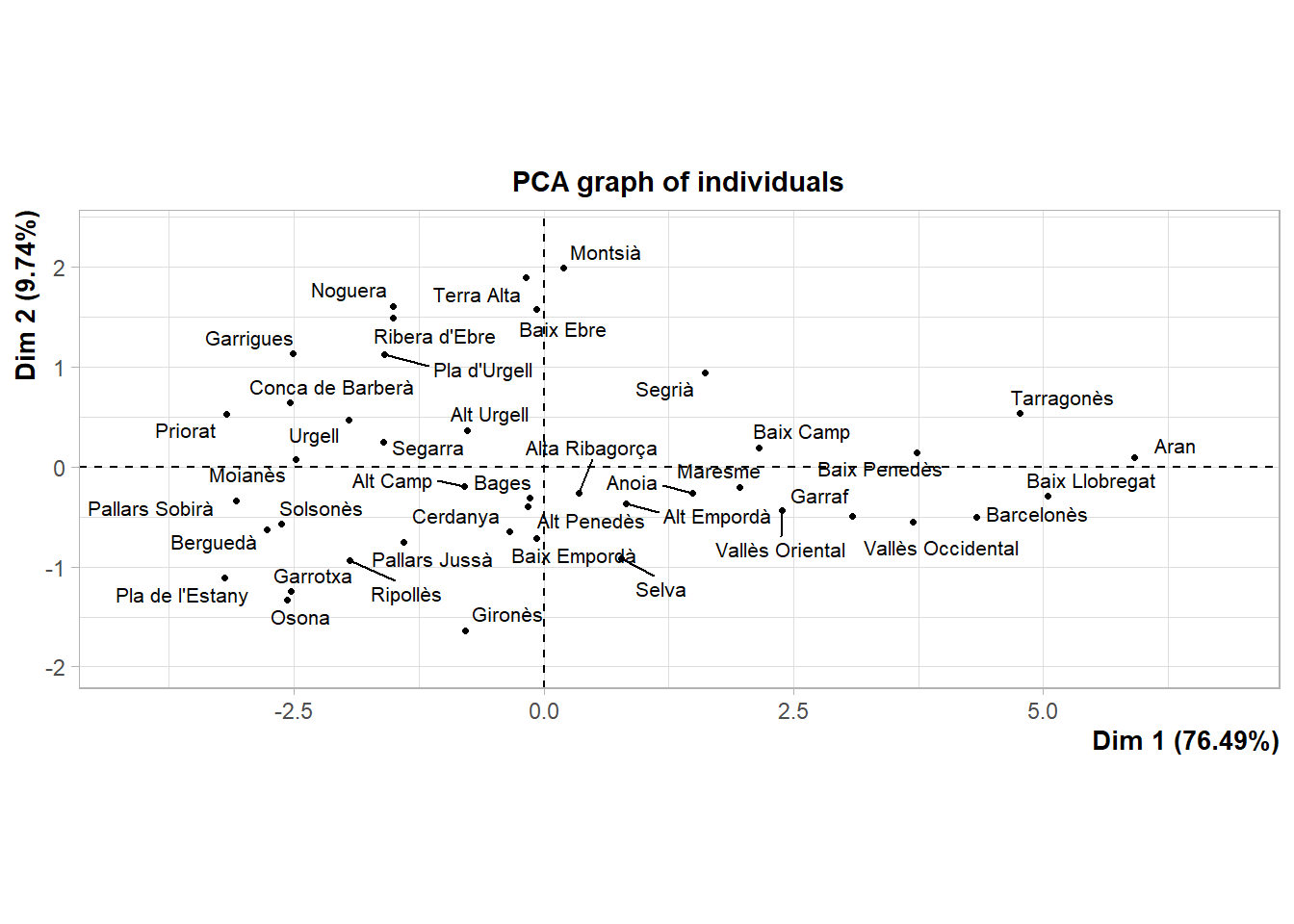

plot(respca_com,choix="var")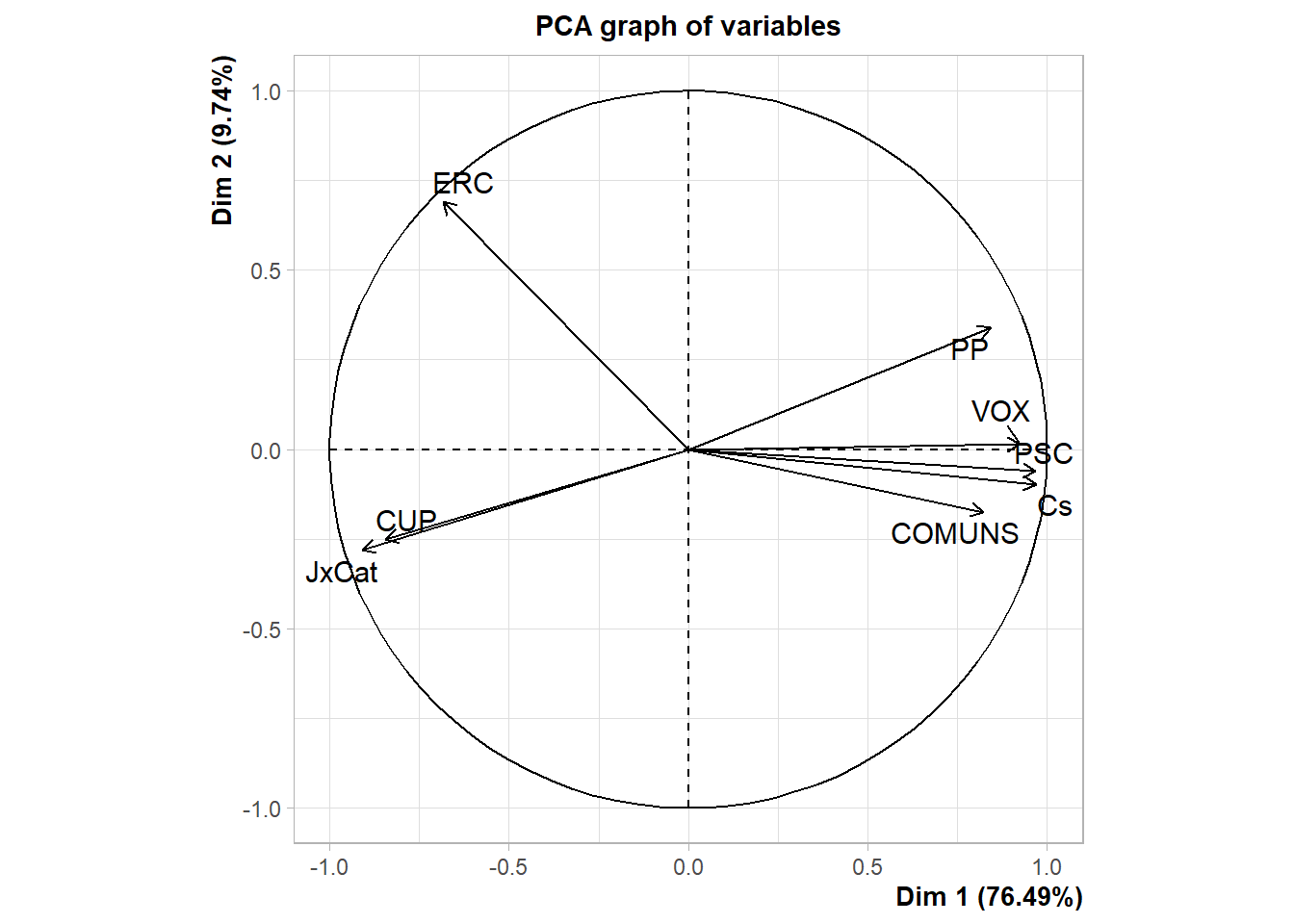

6.3.2 Barómetre (2021-01-29)

Valoració candiadts.

data <- read.spss("http://upceo.ceo.gencat.cat/wsceop/7908/Microdades%20anonimitzades%20-992.sav", to.data.frame = TRUE, use.value.labels = TRUE)

## re-encoding from UTF-8

## Warning in read.spss("http://upceo.ceo.gencat.cat/wsceop/7908/Microdades%20anonimitzades%20-992.sav", : Undeclared level(s) 18, 68,
## 73, 98, 138, 144, 181, 237, 430, 491, 614, 629, 645, 659, 670, 690, 695, 777, 810, 813, 827, 828, 830, 848, 850, 851, 852, 853, 855,
## 877 added in variable: ENQUESTADOR_CODI

## Warning in read.spss("http://upceo.ceo.gencat.cat/wsceop/7908/Microdades%20anonimitzades%20-992.sav", : Undeclared level(s) 1, 2, 3,
## 4, 5, 6, 7, 8, 9 added in variable: P4

## Warning in read.spss("http://upceo.ceo.gencat.cat/wsceop/7908/Microdades%20anonimitzades%20-992.sav", : Undeclared level(s) 1, 2, 3,
## 4, 5, 6, 7, 8, 9 added in variable: P7

## Warning in read.spss("http://upceo.ceo.gencat.cat/wsceop/7908/Microdades%20anonimitzades%20-992.sav", : Undeclared level(s) 1, 2, 3,
## 4, 5, 6, 7, 8, 9 added in variable: P11

## Warning in read.spss("http://upceo.ceo.gencat.cat/wsceop/7908/Microdades%20anonimitzades%20-992.sav", : Undeclared level(s) 1, 2, 3,
## 4, 5, 6, 7, 8, 9 added in variable: P13_A

## Warning in read.spss("http://upceo.ceo.gencat.cat/wsceop/7908/Microdades%20anonimitzades%20-992.sav", : Undeclared level(s) 2, 3, 4,
## 5, 6, 7, 8, 9 added in variable: P13_B

## Warning in read.spss("http://upceo.ceo.gencat.cat/wsceop/7908/Microdades%20anonimitzades%20-992.sav", : Undeclared level(s) 1, 2, 3,
## 4, 5, 6, 7, 8, 9 added in variable: P13_C

## Warning in read.spss("http://upceo.ceo.gencat.cat/wsceop/7908/Microdades%20anonimitzades%20-992.sav", : Undeclared level(s) 1, 2, 3,
## 4, 5, 6, 7, 8, 9 added in variable: P13_D

## Warning in read.spss("http://upceo.ceo.gencat.cat/wsceop/7908/Microdades%20anonimitzades%20-992.sav", : Undeclared level(s) 1, 2, 3,
## 4, 5, 6, 7, 8, 9 added in variable: P13_E

## Warning in read.spss("http://upceo.ceo.gencat.cat/wsceop/7908/Microdades%20anonimitzades%20-992.sav", : Undeclared level(s) 1, 2, 3,
## 4, 5, 6, 7, 8, 9 added in variable: P19B_A_FERNANDEZ

## Warning in read.spss("http://upceo.ceo.gencat.cat/wsceop/7908/Microdades%20anonimitzades%20-992.sav", : Undeclared level(s) 1, 2, 3,
## 4, 5, 6, 7, 8, 9 added in variable: P19B_L_BORRAS

## Warning in read.spss("http://upceo.ceo.gencat.cat/wsceop/7908/Microdades%20anonimitzades%20-992.sav", : Undeclared level(s) 1, 2, 3,
## 4, 5, 6, 7, 8, 9 added in variable: P19B_P_ARAGONES

## Warning in read.spss("http://upceo.ceo.gencat.cat/wsceop/7908/Microdades%20anonimitzades%20-992.sav", : Undeclared level(s) 1, 2, 3,
## 4, 5, 6, 7, 8, 9 added in variable: P19B_S_ILLA

## Warning in read.spss("http://upceo.ceo.gencat.cat/wsceop/7908/Microdades%20anonimitzades%20-992.sav", : Undeclared level(s) 1, 2, 3,
## 4, 5, 6, 7, 8, 9 added in variable: P19B_J_ALBIACH

## Warning in read.spss("http://upceo.ceo.gencat.cat/wsceop/7908/Microdades%20anonimitzades%20-992.sav", : Undeclared level(s) 1, 2, 3,
## 4, 5, 6, 7, 8, 9 added in variable: P19B_C_CARRIZOSA

## Warning in read.spss("http://upceo.ceo.gencat.cat/wsceop/7908/Microdades%20anonimitzades%20-992.sav", : Undeclared level(s) 1, 2, 3,
## 4, 5, 6, 7, 8, 9 added in variable: P19B_D_SABATER

## Warning in read.spss("http://upceo.ceo.gencat.cat/wsceop/7908/Microdades%20anonimitzades%20-992.sav", : Undeclared level(s) 1, 2, 3,
## 4, 5, 6, 7, 8 added in variable: P19B_I_GARRIGA

## Warning in read.spss("http://upceo.ceo.gencat.cat/wsceop/7908/Microdades%20anonimitzades%20-992.sav", : Undeclared level(s) 1, 2, 3,
## 4, 5, 6, 7, 8, 9 added in variable: P19B_A_CHACON

## Warning in read.spss("http://upceo.ceo.gencat.cat/wsceop/7908/Microdades%20anonimitzades%20-992.sav", : Undeclared level(s) 1932,
## 1939, 1942, 1944, 1945, 1946, 1948, 1950, 1951, 1952, 1953, 1954, 1955, 1956, 1957, 1958, 1959, 1960, 1961, 1962, 1963, 1964, 1965,
## 1966, 1967, 1968, 1969, 1970, 1971, 1972, 1973, 1974, 1975, 1976, 1977, 1978, 1979, 1980, 1981, 1982, 1983, 1984, 1985, 1986, 1987,
## 1988, 1989, 1990, 1991, 1992, 1994, 1995, 1996, 1997, 1998, 1999, 2000, 2001, 2002, 2003, 2004, 2005, 2006, 2007, 2008, 2009, 2010,
## 2011, 2013, 2014, 2015, 2016, 2017, 2018, 2019 added in variable: P20

## Warning in read.spss("http://upceo.ceo.gencat.cat/wsceop/7908/Microdades%20anonimitzades%20-992.sav", : Duplicated levels in factor
## P29: Altres

valor <- data %>% 
  mutate(
 FERNANDEZ= ifelse(P19B_A_FERNANDEZ%in%c("No ho sap","No contesta"),NA,as.numeric(P19B_A_FERNANDEZ) -1)
,BORRAS = ifelse(P19B_L_BORRAS%in%c("No ho sap","No contesta"),NA,as.numeric(P19B_L_BORRAS) -1)
,ARAGONES = ifelse(P19B_P_ARAGONES%in%c("No ho sap","No contesta"),NA,as.numeric(P19B_P_ARAGONES) -1)
,ILLA = ifelse(P19B_S_ILLA%in%c("No ho sap","No contesta"),NA,as.numeric(P19B_S_ILLA) -1)
,ALBIACH = ifelse(P19B_J_ALBIACH%in%c("No ho sap","No contesta"),NA,as.numeric(P19B_J_ALBIACH) -1)
,CARRIZOSA = ifelse(P19B_C_CARRIZOSA%in%c("No ho sap","No contesta"),NA,as.numeric(P19B_C_CARRIZOSA) -1)
,SABATER = ifelse(P19B_D_SABATER%in%c("No ho sap","No contesta"),NA,as.numeric(P19B_D_SABATER) -1)
,GARRIGA = ifelse(P19B_I_GARRIGA%in%c("No ho sap","No contesta"),NA,as.numeric(P19B_I_GARRIGA) -1)
,CHACON = ifelse(P19B_A_CHACON%in%c("No ho sap","No contesta"),NA,as.numeric(P19B_A_CHACON) -1)) %>% 
  select(FERNANDEZ,BORRAS,ARAGONES,ILLA,ALBIACH
         ,CARRIZOSA,SABATER,GARRIGA,CHACON)

head(valor)

##   FERNANDEZ BORRAS ARAGONES ILLA ALBIACH CARRIZOSA SABATER GARRIGA CHACON
## 1         0      9        7    6       8         0       2       0      6
## 2        NA     NA       NA    2      NA        NA       6      NA     NA
## 3         5      5        7    8      NA         5      NA      NA      6
## 4        NA      9        8    6      NA         0       8      NA     NA
## 5        NA      8        7    8      NA        NA      NA      NA      6
## 6        NA     NA       NA   NA      NA        NA      NA      NA     NA

library(VIM)

## Loading required package: colorspace

## Loading required package: grid

## VIM is ready to use.

## Suggestions and bug-reports can be submitted at: https://github.com/statistikat/VIM/issues

## 
## Attaching package: 'VIM'

## The following object is masked from 'package:datasets':
## 
##     sleep

aggr(valor)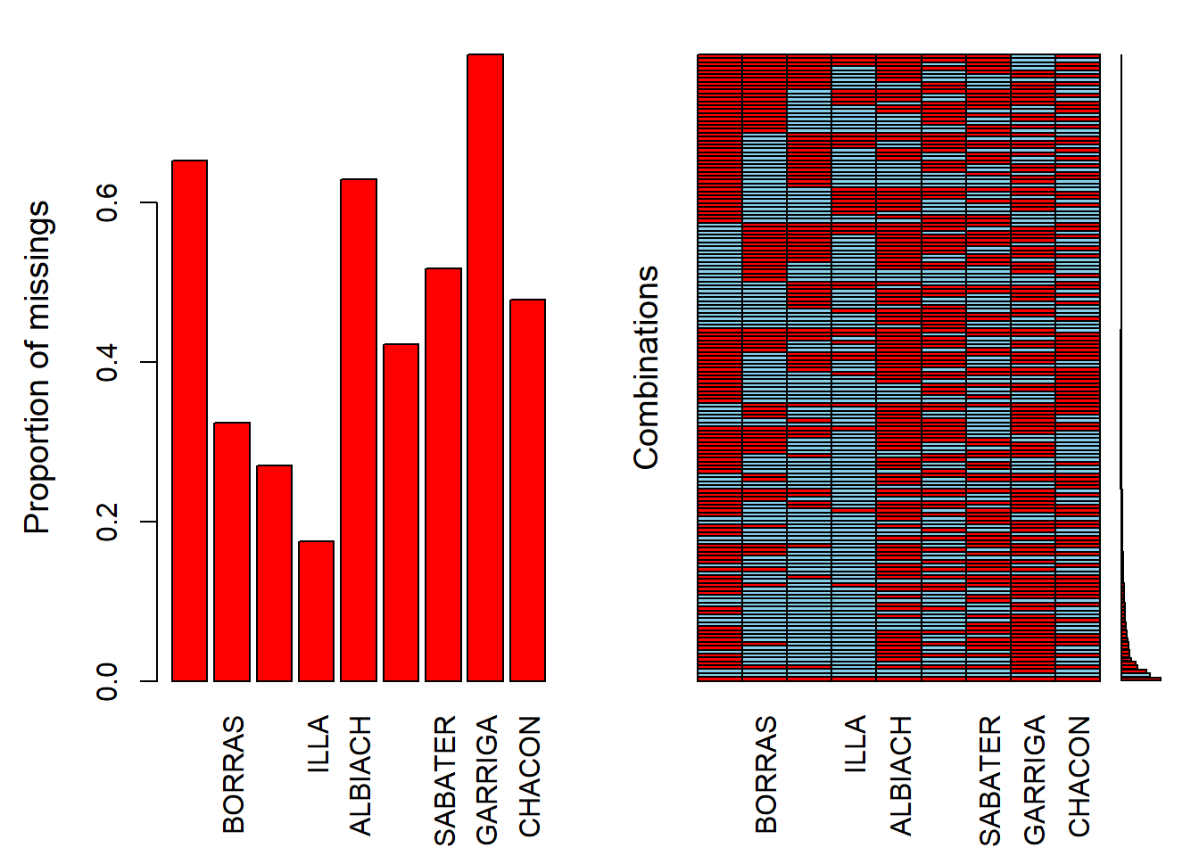

cor()

valorNA<-na.omit(valor)
dim(valorNA)

## [1] 99  9

X <- scale(valorNA)
respca <- PCA(X, graph=FALSE)

summary(respca)

## 
## Call:
## PCA(X = X, graph = FALSE) 
## 
## 
## Eigenvalues
##                        Dim.1   Dim.2   Dim.3   Dim.4   Dim.5   Dim.6   Dim.7   Dim.8   Dim.9
## Variance               3.141   1.883   0.990   0.813   0.550   0.537   0.395   0.379   0.312
## % of var.             34.896  20.926  11.005   9.030   6.109   5.967   4.388   4.206   3.472
## Cumulative % of var.  34.896  55.822  66.828  75.858  81.967  87.934  92.322  96.528 100.000
## 
## Individuals (the 10 first)
##               Dist    Dim.1    ctr   cos2    Dim.2    ctr   cos2    Dim.3    ctr   cos2  
## 1         |  2.890 | -0.162  0.008  0.003 |  1.109  0.659  0.147 | -0.937  0.895  0.105 |
## 21        |  2.884 |  0.818  0.215  0.080 | -0.311  0.052  0.012 | -1.757  3.147  0.371 |
## 23        |  2.410 | -0.343  0.038  0.020 |  2.004  2.154  0.691 |  0.689  0.484  0.082 |
## 27        |  2.466 |  1.124  0.406  0.208 |  0.072  0.003  0.001 |  0.006  0.000  0.000 |
## 28        |  3.314 |  2.829  2.575  0.729 |  0.301  0.049  0.008 | -0.603  0.370  0.033 |
## 33        |  1.980 | -0.361  0.042  0.033 |  0.286  0.044  0.021 |  0.216  0.048  0.012 |
## 43        |  2.576 |  1.841  1.090  0.510 |  0.103  0.006  0.002 | -0.947  0.915  0.135 |
## 82        |  3.848 |  3.223  3.340  0.701 | -1.757  1.655  0.208 |  0.727  0.538  0.036 |
## 92        |  1.669 | -0.821  0.217  0.242 | -0.032  0.001  0.000 | -0.233  0.056  0.020 |
## 110       |  3.709 | -1.964  1.241  0.280 |  1.351  0.978  0.133 | -0.392  0.157  0.011 |
## 
## Variables
##              Dim.1    ctr   cos2    Dim.2    ctr   cos2    Dim.3    ctr   cos2  
## FERNANDEZ |  0.616 12.092  0.380 | -0.572 17.359  0.327 |  0.232  5.426  0.054 |
## BORRAS    |  0.351  3.923  0.123 |  0.642 21.911  0.413 |  0.375 14.230  0.141 |
## ARAGONES  |  0.662 13.951  0.438 |  0.442 10.378  0.195 | -0.094  0.883  0.009 |
## ILLA      |  0.627 12.534  0.394 |  0.032  0.053  0.001 | -0.658 43.664  0.432 |
## ALBIACH   |  0.759 18.362  0.577 |  0.229  2.796  0.053 | -0.337 11.438  0.113 |
## CARRIZOSA |  0.630 12.640  0.397 | -0.589 18.425  0.347 |  0.036  0.132  0.001 |
## SABATER   |  0.413  5.430  0.171 |  0.548 15.919  0.300 |  0.207  4.326  0.043 |
## GARRIGA   |  0.572 10.432  0.328 | -0.486 12.526  0.236 |  0.214  4.609  0.046 |
## CHACON    |  0.578 10.635  0.334 |  0.109  0.634  0.012 |  0.389 15.293  0.151 |

plot(respca,choix="ind", cex=0.7)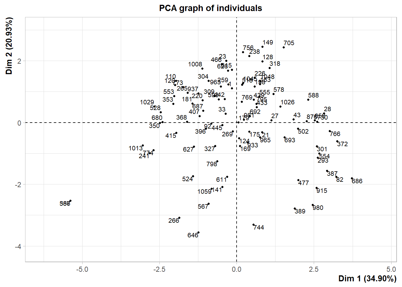

plot(respca,choix="var")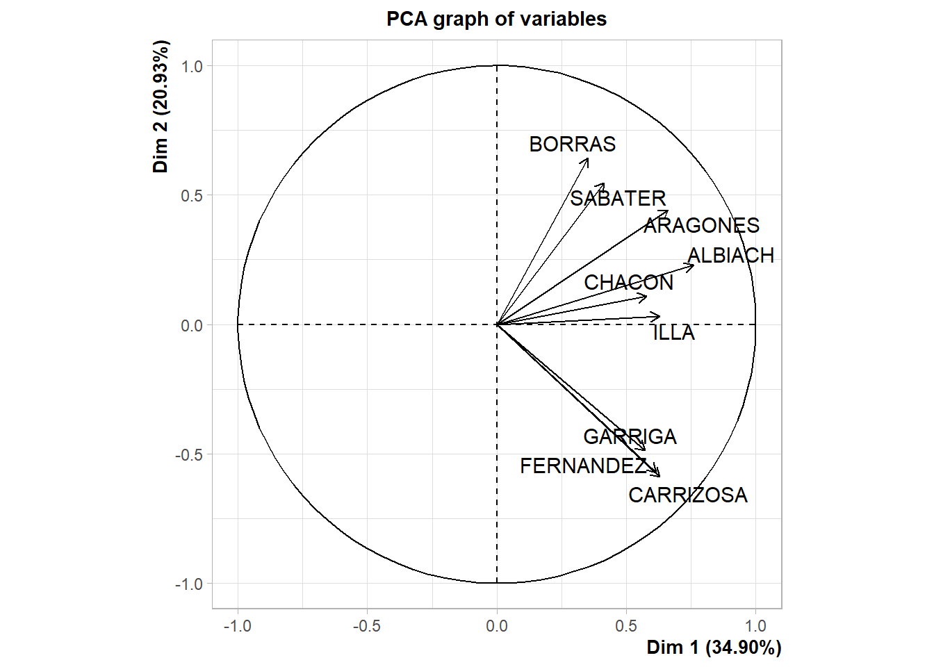

6.4 Analisis Factorial amb dades omeses

fit = factanal(X, factors=2,rotation = 'varimax')
fit

## 
## Call:
## factanal(x = X, factors = 2, rotation = "varimax")
## 
## Uniquenesses:
## FERNANDEZ    BORRAS  ARAGONES      ILLA   ALBIACH CARRIZOSA   SABATER   GARRIGA    CHACON 
##     0.391     0.713     0.435     0.666     0.427     0.295     0.729     0.578     0.760 
## 
## Loadings:
##           Factor1 Factor2
## FERNANDEZ  0.779         
## BORRAS    -0.120   0.522 
## ARAGONES   0.122   0.742 
## ILLA       0.335   0.472 
## ALBIACH    0.317   0.687 
## CARRIZOSA  0.838         
## SABATER            0.520 
## GARRIGA    0.643         
## CHACON     0.282   0.401 
## 
##                Factor1 Factor2
## SS loadings      2.045   1.962
## Proportion Var   0.227   0.218
## Cumulative Var   0.227   0.445
## 
## Test of the hypothesis that 2 factors are sufficient.
## The chi square statistic is 28.5 on 19 degrees of freedom.
## The p-value is 0.0742

attributes(fit)

## $names
##  [1] "converged"    "loadings"     "uniquenesses" "correlation"  "criteria"     "factors"      "dof"          "method"      
##  [9] "rotmat"       "STATISTIC"    "PVAL"         "n.obs"        "call"        
## 
## $class
## [1] "factanal"

A=fit$loadings; ma=max(abs(A)) 
L<-A[,1:2]
comm <-  apply(A[,1:2]**2, 1,sum)
factvar <-  apply(A[,1:2]**2, 2,sum)
unique <- 1 - comm
LL<- cbind(L, communalities=comm, uniq= unique)
LLL <- rbind(LL, c(factvar,sum(comm), sum(unique) )  )

round(LLL,digits=3)

##           Factor1 Factor2 communalities  uniq
## FERNANDEZ   0.779   0.048         0.609 0.391
## BORRAS     -0.120   0.522         0.287 0.713
## ARAGONES    0.122   0.742         0.565 0.435
## ILLA        0.335   0.472         0.334 0.666
## ALBIACH     0.317   0.687         0.573 0.427
## CARRIZOSA   0.838   0.049         0.705 0.295
## SABATER    -0.033   0.520         0.271 0.729
## GARRIGA     0.643   0.093         0.422 0.578
## CHACON      0.282   0.401         0.240 0.760
##             2.045   1.962         4.006 4.994

6.4.1 Representació de les variables

plot(A[,1],A[,2], xlim = c(-ma, ma), ylim = c(-ma,ma), type = 'n', xlab="factor 1", ylab="factor 2") 
arrows(rep(0,6), rep(0,6), A[,1], A[,2], length = 0.05) 
abline(h = 0, lty = 3) 
abline(v = 0, lty = 3) 
text(A[,1], A[,2] , colnames(X), cex =.7)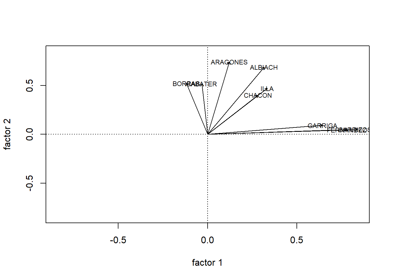 

6.4.2 Anàlisis factorial amb correlacions dos a dos

head(valor)

##   FERNANDEZ BORRAS ARAGONES ILLA ALBIACH CARRIZOSA SABATER GARRIGA CHACON
## 1         0      9        7    6       8         0       2       0      6
## 2        NA     NA       NA    2      NA        NA       6      NA     NA
## 3         5      5        7    8      NA         5      NA      NA      6
## 4        NA      9        8    6      NA         0       8      NA     NA
## 5        NA      8        7    8      NA        NA      NA      NA      6
## 6        NA     NA       NA   NA      NA        NA      NA      NA     NA

dim(valor)

## [1] 1100    9

aggr(valor)

R <-  cor(valor, use="pairwise.complete.obs")
round(R,3)

##           FERNANDEZ BORRAS ARAGONES  ILLA ALBIACH CARRIZOSA SABATER GARRIGA CHACON
## FERNANDEZ     1.000  0.005    0.074 0.231   0.327     0.726   0.120   0.648  0.350
## BORRAS        0.005  1.000    0.517 0.205   0.308    -0.067   0.534   0.012  0.380
## ARAGONES      0.074  0.517    1.000 0.439   0.504     0.030   0.408   0.030  0.463
## ILLA          0.231  0.205    0.439 1.000   0.497     0.214   0.310   0.209  0.402
## ALBIACH       0.327  0.308    0.504 0.497   1.000     0.229   0.422   0.317  0.467
## CARRIZOSA     0.726 -0.067    0.030 0.214   0.229     1.000   0.005   0.605  0.283
## SABATER       0.120  0.534    0.408 0.310   0.422     0.005   1.000   0.158  0.443
## GARRIGA       0.648  0.012    0.030 0.209   0.317     0.605   0.158   1.000  0.258
## CHACON        0.350  0.380    0.463 0.402   0.467     0.283   0.443   0.258  1.000

fit = factanal(covmat =R, factors=2,rotation = 'varimax')
A=fit$loadings; ma=max(abs(A)) 

Veiem la representació.

L<-A[,1:2]
comm <-  apply(A[,1:2]**2, 1,sum)
factvar <-  apply(A[,1:2]**2, 2,sum)
unique <- 1 - comm
LL<- cbind(L, communalities=comm, uniq= unique)
LLL <- rbind(LL, c(factvar,sum(comm), sum(unique) )  )
round(LLL,3)

##           Factor1 Factor2 communalities  uniq
## FERNANDEZ   0.129   0.868         0.769 0.231
## BORRAS      0.649  -0.106         0.433 0.567
## ARAGONES    0.750  -0.020         0.563 0.437
## ILLA        0.531   0.218         0.330 0.670
## ALBIACH     0.643   0.286         0.495 0.505
## CARRIZOSA   0.028   0.830         0.689 0.311
## SABATER     0.651   0.031         0.425 0.575
## GARRIGA     0.117   0.727         0.542 0.458
## CHACON      0.628   0.302         0.485 0.515
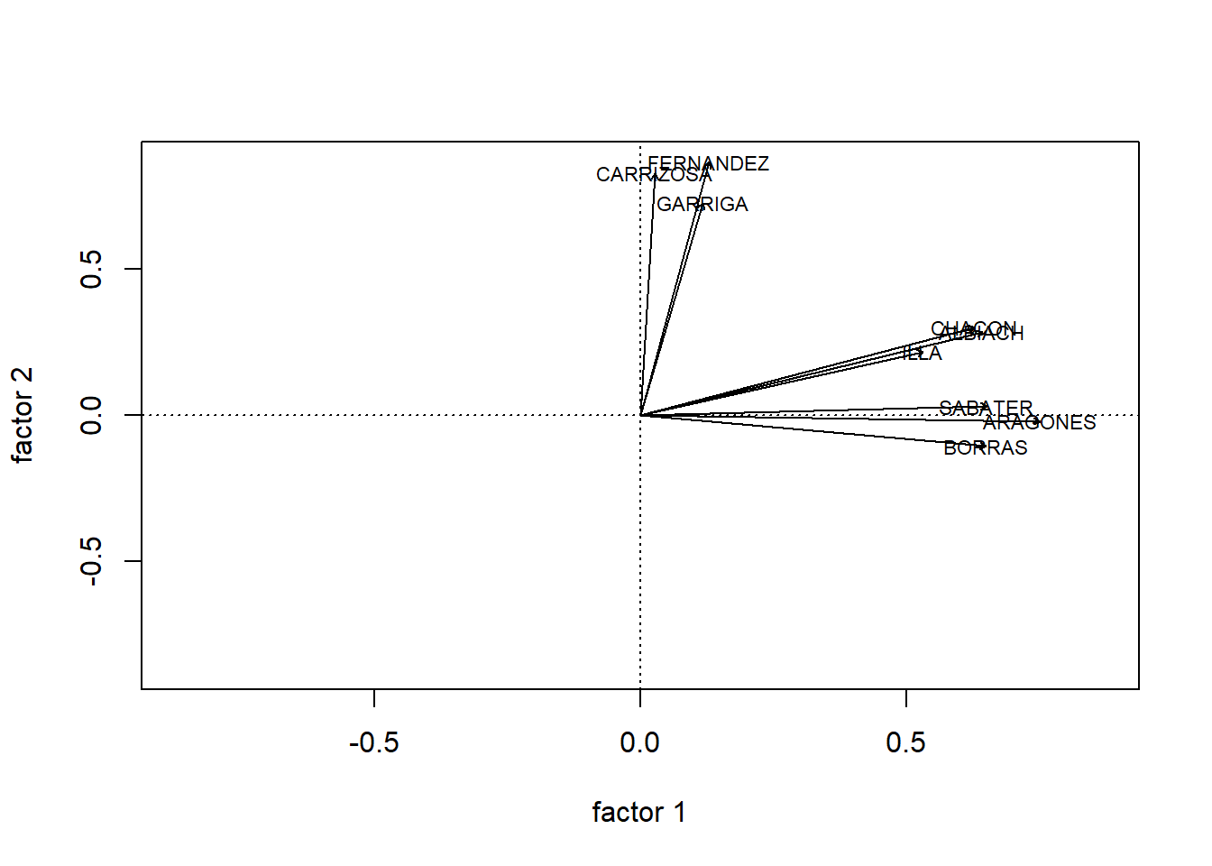
##             2.529   2.203         4.732 4.268

Gráficament.

plot(A[,1],A[,2], xlim = c(-ma, ma), ylim = c(-ma,ma), type = 'n', xlab="factor 1", ylab="factor 2") 
arrows(rep(0,6), rep(0,6), A[,1], A[,2], length = 0.04) 
abline(h = 0, lty = 3) 
abline(v = 0, lty = 3) 
text(A[,1], A[,2] , rownames(R), cex =.7)